Phase portrait plotter: generator, center, spiral, and saddle
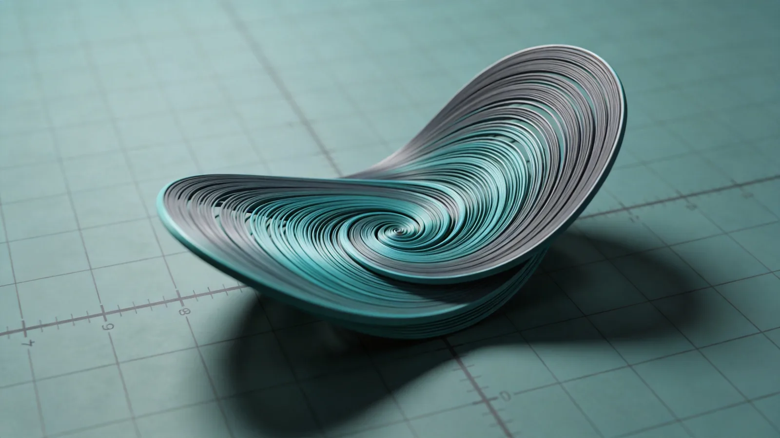
A phase portrait is a geometric representation of a dynamical system: a set of first-order differential equations whose solutions trace curves through a state space. For a two-dimensional autonomous system, the state at any instant is a point (x, y) and the rate of change is given by a vector field (dx/dt, dy/dt). Plotting this field together with representative solution trajectories reveals how the system evolves from different initial conditions without solving the equations analytically.
Phase portraits are central to the study of ordinary differential equations in mathematics, physics, and engineering. In population ecology, the Lotka–Volterra equations model predator–prey dynamics; their phase portrait shows closed orbits around a coexistence equilibrium. In classical mechanics, a pendulum's angle and angular velocity form a two-dimensional state, and the portrait displays spirals toward a stable rest point or closed loops for undamped oscillation. Electrical circuits with inductors and capacitors exhibit analogous behavior.
Equilibrium points—where dx/dt = dy/dt = 0—are the landmarks of a phase portrait. Linearizing the system near each equilibrium and examining the eigenvalues of the Jacobian matrix classifies the local behavior as a node, saddle, spiral, or center. A stable node attracts nearby trajectories; a saddle has one stable and one unstable direction; a spiral combines rotation with approach or departure. These classifications appear on every differential equations exam and in research on nonlinear dynamics.
Students first encounter phase portraits when learning to interpret vector fields and nullclines. The x-nullcline is where dx/dt = 0; the y-nullcline is where dy/dt = 0. Their intersections are equilibria, and the regions between nullclines indicate whether each variable is increasing or decreasing. Sketching nullclines by hand builds intuition before relying on software, but numerical tools accelerate exploration of parameter changes.
The Phase Portrait Generator on Online Science Tools is a phase portrait calculator and plotter: it accepts a pair of differential equations, plots the vector field on an adjustable domain, and integrates trajectories from clicks on the plane. Built-in portraits include a center (closed orbits), stable and unstable spirals, a saddle, stable and unstable nodes, a damped pendulum, Van der Pol, and predator–prey. Use it alongside the 2D Graphing Calculator for one-dimensional function plots and the Linear Equations Solver when linearizing systems near equilibria.
- Autonomous systems: dx/dt and dy/dt depend only on (x, y), not explicitly on time
- Equilibrium points occur where both rate equations equal zero simultaneously
- Jacobian eigenvalues at an equilibrium determine local stability classification
- Nullclines partition the plane into regions of increasing and decreasing x and y
Formulas you will actually use
A two-dimensional autonomous system is defined by a pair of coupled first-order ODEs. The vector field, equilibrium conditions, and linearization Jacobian form the analytical backbone of phase portrait analysis.
System:
  dx/dt = f(x, y)
  dy/dt = g(x, y)

Vector field at each point (x, y):
  v = (f(x, y), g(x, y))

Equilibrium (x*, y*):
  f(x*, y*) = 0  and  g(x*, y*) = 0

Jacobian matrix (for linearization):
  J = | ∂f/∂x   ∂f/∂y |
      | ∂g/∂x   ∂g/∂y |

Eigenvalues λ of J at (x*, y*) classify stability:
  λ₁, λ₂ both real, same sign  →  node (stable if negative)
  λ₁, λ₂ real, opposite signs   →  saddle (unstable)
  λ = α ± iβ, α ≠ 0             →  spiral (stable if α < 0)
λ = ± iβ (pure imaginary) → center (neutrally stable)- Trajectories are tangent to the vector field at every point and never cross (except at equilibria) by uniqueness of solutions.
- For non-autonomous systems with explicit time dependence, augment the state space or use the Time Graphing Tool instead.
- Numerical integration (e.g., Runge–Kutta) approximates trajectories when closed-form solutions are unavailable.
Step-by-step example: Phase Portrait of a Damped Pendulum
Model a pendulum with damping: dx/dt = y, dy/dt = −sin(x) − 0.5y, where x is the angle and y is angular velocity. Identify equilibria and describe the expected portrait near the origin.
- Set dx/dt = 0: y = 0. Set dy/dt = 0: −sin(x) − 0.5y = 0, so with y = 0, sin(x) = 0.
- Equilibria: (0, 0), (π, 0), (−π, 0), and all integer multiples of π along y = 0.
- Linearize at the origin: f = y, g = −sin(x) − 0.5y. At (0,0): ∂f/∂x = 0, ∂f/∂y = 1, ∂g/∂x = −cos(0) = −1, ∂g/∂y = −0.5.
- Jacobian at origin: J = [[0, 1], [−1, −0.5]].
- Characteristic equation: λ² + 0.5λ + 1 = 0. Discriminant: 0.25 − 4 = −3.75 < 0.
- Complex eigenvalues with real part −0.25: the origin is a stable spiral. Trajectories spiral inward toward (0, 0).
- At (π, 0): cos(π) = −1, so ∂g/∂x = 1. Jacobian has eigenvalues with opposite signs → saddle point.
Enter dx/dt = y and dy/dt = -sin(x) - 0.5*y into the Phase Portrait Generator on Online Science Tools. Set the viewing window to x ∈ [−4, 4] and y ∈ [−3, 3], then click near (0.5, 0) to launch a trajectory. You should see a spiral converging to the origin, confirming the stable spiral classification. Launch another trajectory near (3.5, 0) to observe the saddle behavior at x = π. Compare vector field directions with your nullcline sketch.
Frequently asked questions
Is this a phase portrait calculator, generator, and plotter?
Yes. The Phase Portrait Generator is a phase portrait calculator and phase portrait plotter for 2D autonomous systems dx/dt = f(x, y), dy/dt = g(x, y). Enter the two equations (or pick a preset such as center, stable spiral, or saddle), then click the plane to integrate trajectories. Equilibria are classified as node, saddle, spiral, or center from a numerical Jacobian.
What is a center vs a stable spiral in a phase portrait?
A center has purely imaginary eigenvalues: nearby trajectories are closed orbits that neither approach nor leave the equilibrium (try the Center preset, dx/dt = −y, dy/dt = x). A stable spiral has complex eigenvalues with a negative real part: trajectories rotate while spiraling inward (try Spiral Sink). An unstable spiral spirals outward. Enable “Show equilibria + classification” to label the type at each equilibrium.
What is the difference between a phase portrait and a regular graph?
A regular graph plots a dependent variable against an independent variable, such as y versus x for a function. A phase portrait plots one state variable against another state variable (y versus x) with time as an implicit parameter along each curve. Multiple trajectories can pass through different regions of the same plane, and the vector field shows instantaneous direction at every point. The 2D Graphing Calculator handles explicit functions; the Phase Portrait Generator handles coupled differential equations.
Why do trajectories never cross in a phase portrait?
By the existence and uniqueness theorem for ordinary differential equations, a given initial condition (x₀, y₀) determines exactly one solution curve. If two trajectories crossed at a point, that point would serve as two different initial conditions for the same system, violating uniqueness. The only exception is equilibrium points, where the velocity vector is zero and trajectories can meet.
How do I find and classify equilibrium points?
Solve the simultaneous equations f(x, y) = 0 and g(x, y) = 0. At each solution, compute the Jacobian matrix of partial derivatives and find its eigenvalues. Real eigenvalues of the same sign indicate a node; opposite signs indicate a saddle; complex eigenvalues indicate a spiral or center depending on whether the real part is nonzero. In the Phase Portrait Generator, look for places where arrows shrink to zero, or launch nearby trajectories to see whether they approach or leave a candidate equilibrium.
Can I use phase portraits for systems with three or more variables?
Phase portraits as two-dimensional plots require a two-dimensional state space. For three or more variables, you can project onto a two-dimensional slice (fixing other coordinates) or examine two-variable subsystems. Higher-dimensional analysis uses tools like Lyapunov exponents and bifurcation diagrams. The Phase Portrait Generator is designed specifically for 2D autonomous systems, which cover the majority of introductory differential equations coursework.
References & further reading
Standards bodies, university open courseware, and peer-reviewed references that align with the methods used on this page.
Keep learning with chemistry calculators, the math tools, and study guides on Online Science Tools.