What is the 2D Graphing Calculator?
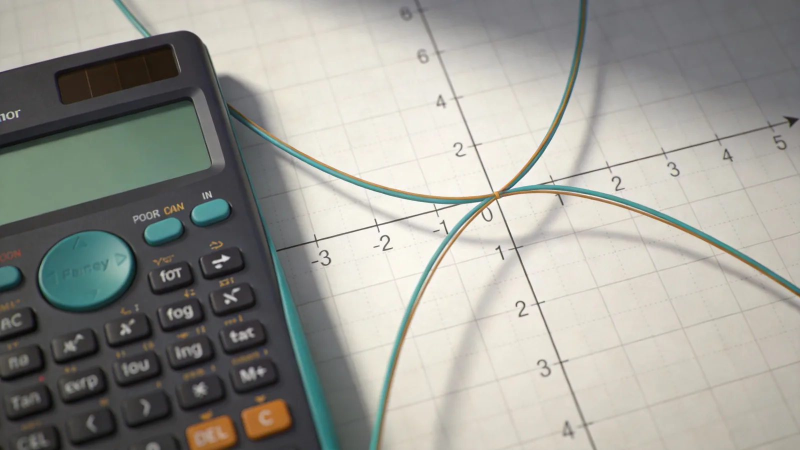
A graphing calculator plots the relationship between an independent variable x and a dependent output f(x), turning an algebraic expression into a visual curve on the coordinate plane. By displaying the shape, intercepts, turning points, and asymptotic behavior of a function, graphing reveals properties that are difficult to detect from the formula alone. The graph of f(x) = x³ − 3x, for instance, immediately shows two local extrema and three x-intercepts that would require calculus or factoring to find analytically.
Function graphing is a foundational skill in algebra, precalculus, calculus, and applied mathematics. Before the derivative is formally defined, students use graphs to estimate slopes and identify increasing and decreasing intervals. In calculus, graphs confirm analytical results: a critical point where f′(x) = 0 should appear as a horizontal tangent on the graph. In physics, position–time or velocity–time graphs connect mathematical functions to measurable quantities.
The viewing window— the range of x and y values displayed— critically affects what you see. A function with rapid growth may look flat in a wide window but reveal detail when zoomed in. Local extrema detection algorithms sample the function numerically to find points where the sign of the slope changes, approximating where the derivative equals zero. These automated features complement hand calculations and help students verify their work.
Graphing also supports comparing multiple functions on the same axes. Overlaying y = sin(x) and y = cos(x) shows their phase relationship; plotting a function and its tangent line at a point illustrates the derivative geometrically. Inequalities become regions: shading above or below a curve represents solution sets for y > f(x) or y < f(x).
The 2D Graphing Calculator on Online Science Tools accepts standard mathematical expressions, renders them on an interactive canvas with pan and zoom, and highlights local maxima and minima automatically. Pair it with the Linear Equations Solver for systems whose solutions are intersection points of lines, or with the Time Graphing Tool when the function depends on time as well as position.
- The graph of y = f(x) consists of all points (x, f(x)) in the plane
- x-intercepts occur where f(x) = 0; y-intercepts occur at f(0)
- Local maxima and minima appear where the slope changes sign (f′(x) = 0 or undefined)
- Transformations (shifts, stretches, reflections) modify the graph predictably
Formulas you will actually use
Graphing relies on evaluating f(x) at sample points and connecting them. Key analytical formulas help locate intercepts, extrema, and asymptotes before or after plotting.
Function:  y = f(x)

x-intercepts:  solve f(x) = 0
y-intercept:   (0, f(0))

Slope (derivative):
  f′(x) = lim(h→0) [f(x+h) − f(x)] / h

Critical points:  f′(x) = 0  or  f′(x) undefined

Second derivative test:
  f″(x) > 0  →  local minimum at x
  f″(x) < 0  →  local maximum at x

Common transformations of f(x):
  f(x) + k       vertical shift up by k
  f(x − h)       horizontal shift right by h
  a·f(x)         vertical stretch by |a|
f(b·x) horizontal compression by 1/|b|- Vertical asymptotes occur where f(x) → ±∞; horizontal asymptotes describe end behavior as x → ±∞.
- Numerical plotting samples f at discrete x values; too few points may miss sharp features or oscillations.
- Piecewise functions require separate expressions over each domain interval.
Step-by-step example: Graphing and Analyzing f(x) = x³ − 3x
Analyze and sketch the cubic function f(x) = x³ − 3x. Find intercepts, critical points, and classify each extremum.
- y-intercept: f(0) = 0, so the graph passes through the origin.
- x-intercepts: x³ − 3x = x(x² − 3) = 0, so x = 0, x = √3 ≈ 1.732, x = −√3 ≈ −1.732.
- Derivative: f′(x) = 3x² − 3 = 3(x² − 1). Set f′(x) = 0: x = ±1.
- Evaluate: f(1) = 1 − 3 = −2 (local minimum); f(−1) = −1 + 3 = 2 (local maximum).
- Second derivative: f″(x) = 6x. f″(1) = 6 > 0 confirms minimum; f″(−1) = −6 < 0 confirms maximum.
- End behavior: as x → +∞, f(x) → +∞; as x → −∞, f(x) → −∞.
- Sketch: rising from lower left, peak at (−1, 2), descending through origin, minimum at (1, −2), then rising to upper right.
Enter x^3 - 3*x into the 2D Graphing Calculator on Online Science Tools and set the window to x ∈ [−3, 3], y ∈ [−4, 4]. The tool should display the cubic curve passing through the three x-intercepts and automatically detect local extrema near (−1, 2) and (1, −2). Compare the detected coordinates to your analytical results. For a related system of lines, use the Linear Equations Solver to find where two linear functions intersect.
Frequently asked questions
Why does my graph look wrong or incomplete?
The most common cause is an inappropriate viewing window. If the function grows rapidly, most of the curve may be compressed into a corner of the screen. Try narrowing the x-range or adjusting the y-range. Another cause is a domain restriction: functions like sqrt(x) or 1/x are undefined at certain x values, creating gaps or asymptotes that require the window to include both sides of the discontinuity.
How does the calculator find local extrema automatically?
The 2D Graphing Calculator samples the function at many points across the visible window and looks for sign changes in the approximate slope between adjacent samples. When the slope changes from positive to negative, a local maximum is flagged; from negative to positive, a local minimum. This numerical method approximates solving f′(x) = 0 and works for any differentiable function, though very sharp peaks may require a narrower window for accurate detection.
Can I graph multiple functions at once?
Yes. Enter additional expressions to overlay them on the same axes. This is useful for comparing a function to its derivative estimate, finding intersection points visually, or exploring families of curves with different parameters. Intersection points of two graphs f(x) and g(x) correspond to solutions of f(x) = g(x).
What functions can the graphing calculator handle?
The 2D Graphing Calculator supports polynomials, trigonometric functions (sin, cos, tan), exponentials, logarithms, absolute value, square roots, and combinations via standard arithmetic operators. Nested expressions and common constants like pi and e are recognized. For parametric or time-dependent curves, switch to the Time Graphing Tool, which handles x(t) and y(t) parameterizations.
References & further reading
Standards bodies, university open courseware, and peer-reviewed references that align with the methods used on this page.
Keep learning with chemistry calculators, the math tools, and study guides on Online Science Tools.